
You can calculate fields in LibreOffice Calc by adding a custom formula to a pivot table. The calculated column becomes part of the table, alongside your existing data fields.
We use sales data to work with gross profit and profit margin. First, we’ll set up the pivot table so you can filter the data by salesperson and review each region separately.
Set up a pivot table to calculate fields in LibreOffice Calc
Pivot tables take large amounts of data and let you summarize and analyze specific parts of it. In our example, we want sales and cost totals for each region.
Select the source data
Let’s start with the basics of creating a Pivot table in LibreOffice.
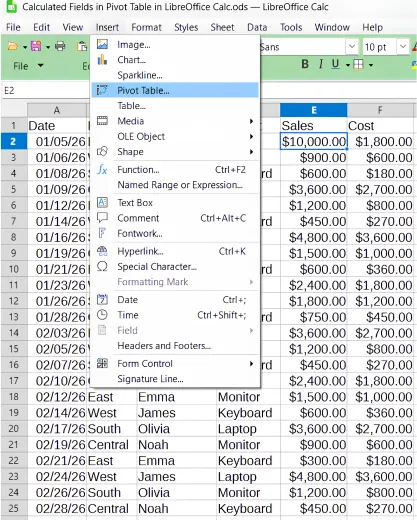
- Select any cell within your sales data.
- Choose Insert > Pivot Table.
- In the Select Source box, leave Current Selection selected if Calc has selected the full data set.
- Choose OK to open the pivot table layout.
The available fields match your column headers. We use those fields to tell Calc how to lay out the table.
Arrange the fields and choose a destination
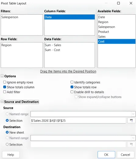
- Drag Salesperson into Filter so you can display data for selected salespeople.
- Leave the default Data field in Column. This tells Calc to display the data fields as columns.
- Drag Region into Row so each region appears on its own row.
- Drag Sales and Cost into Data Fields.
- Leave the row and column totals enabled.
- Under Source and Destination, choose New Sheet as the destination, then select OK.
We keep our pivot table on a new sheet to separate it from the raw data. You can choose a location in the current sheet instead.
Filter the sales data and adjust the layout
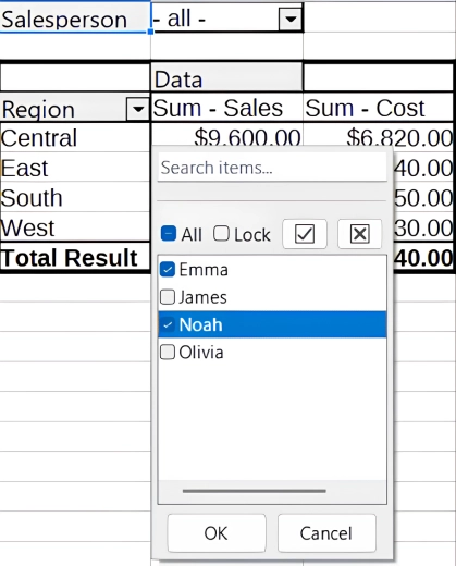
Our pivot table now shows sales and cost by region. LibreOffice describes pivot tables as interactive summaries. They filters let you narrow down which data fields appear in Calc.
Show selected salespeople or regions
- Open the Salesperson filter and select the salespeople you want to include. You can select more than one.
- Choose All when you want to show everyone’s data again.
- Open the Region drop-down, clear the current selection, and select South.
- Choose OK to show only the South region. Select all regions again to restore the full view.
Reopen the pivot table layout
- Select a cell inside the pivot table.
- Right-click and choose Properties.
- Adjust the fields or settings in the layout, then choose OK.
This brings you back to the same layout window we used during setup.
Open the calculated-field controls
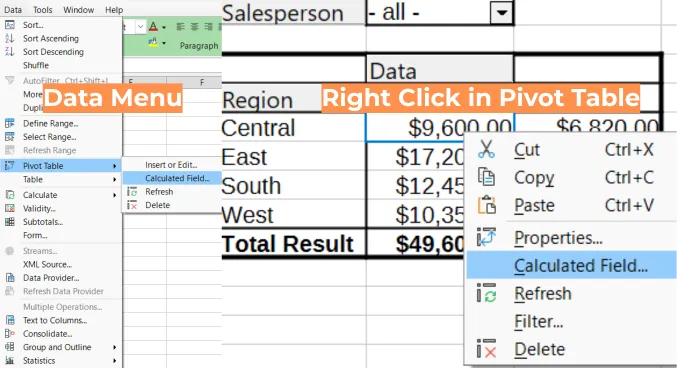
With our sales data in place, we want to know our gross profit and profit margin. LibreOffice’s calculated-field documentation describes a calculated field as a new data column with a custom formula that becomes part of the pivot table.
Use the menu to calculate fields in LibreOffice Calc
- Select any cell inside your pivot table.
- Open Data > Pivot Table.
- Choose Calculated Fields to open the Insert Calculated Fields box.
You can also right-click a cell inside the pivot table and choose Calculated Fields. Both routes open the same controls.
Name the calculated fields
We name our first calculated field Gross Profit and our second Profit Margin Percent. The formula box is where we tell Calc exactly what we want it to do.
Define the formula
This is where we tell Calc what we are calculating.
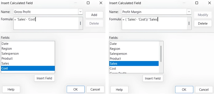
- Enter Formula for Gross Profit
- Click Sales > Insert Field > – > Click Cost > Insert Field > Okay
- Repeat for Profit Margin
- Enter ( > Click Sales > Insert Field > – Click Cost > ) > / > Click Sales > Okay
The Add button lets you work with multiple calculated fields in the dialog. We handle them one at a time so each calculation is separate.
As calculated fields are added, Calc automatically includes them in Data Fields. You can see them alongside Sales and Cost when you reopen Properties.
For the Excel workflow, our guide to Excel pivot table calculations covers that application’s calculated-field controls.
Keep calculated fields within the Calc pivot table
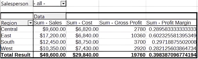
When you calculate fields in LibreOffice Calc, the custom columns become part of the pivot table. In our sales example, that puts gross profit and profit margin alongside sales and cost.
We use the layout to organize those fields and the filters to focus on selected salespeople or regions. The calculations and the summarized data stay together in the same table.
Get Started with Microsoft 365 or LibreOffice.
Be sure to subscribe to my YouTube Channel for more Microsoft 365 and LibreOffice Tutorials.
This page may contain affiliate links. These are tools I personally use and love. I may receive a small commission should you make a purchase using one of these links. This helps keep the tutorials and website posts coming and up to date. Thank you for your support! For more information please see my full disclaimer.